Last article, we introduced linear regression and applied it to predict MLB teams’ runs scored given OPS. Linear regression is great at predicting numerical values. For example, it can predict runs scored given OPS. However, what happens if we want to move away from predicting continuous values and do binary classification? How can we predict whether a batter’s swing mechanics will result in a “hard-hit” batted ball? We are going to have to turn to logistic regression!
Contrary to its name, logistic regression is a classification technique (you will see where the regression part comes from). Logistic regression involves a probabilistic view of classification. This binary classification method maps a data point to a probabilistic value in the range 0 to 1. Let’s dig into some mathematical formalities.
Logistic Regression
Preliminaries
“Never tell me the odds” - Han Solo.
The average movie watcher could hear this quote with a slight alteration, where the word “odds” is replaced by “probability,” and they would not bat an eye. However, a statistician would have an issue with substituting the word “odds” with “probability.” While in layman terms they both share similar meaning, in mathematics they are defined distinctly.
Odds are a transformation of probabilities - they are another way to think about probabilities. More formally, \text{odds} = \frac{p}{1-p}
where p denotes some probability value between 0 and 1, and 1-p denotes the complement. Think of it as the probability of something happening divided by the probability of it not happening. If given some event, E, where the odds are x to y, then that means Odds(E)=\frac{x}{y}. Subsequently, P(E)=\frac{x}{x+y}. The range of possible values for odds becomes 0 to \infty. When using probability values between 0 and 1, the range of odds becomes (0,1). Observe that this is an open interval. If p=1, then the denominator becomes 1-1 = 0. We cannot divide by zero, so the upper bound is undefined at 1. When p=0, we get \frac{0}{1}=0. If we are going to do any regressions of this sort, we will need to expand our real number bounds.
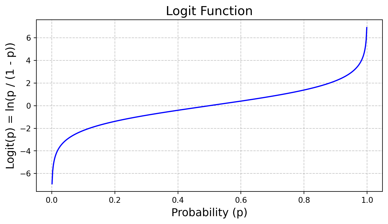
To get an unbounded range, we introduce the logit function. The logit function takes in a value between 0 and 1 and maps it to a value between -\infty and \infty.
z = \log_e{\frac{p}{1-p}}.
Below is a plot for what the logit function looks like.
Code
import numpy as npimport pandas as pdimport seaborn as snsimport matplotlib.pyplot as plt# x valuesp = np.linspace(0.001, 0.999, 500)# calculate the logit function. np uses base e by default.logit_p = np.log(p / (1- p))data = pd.DataFrame({'Probability (p)': p, 'Logit(p)': logit_p})# plottingplt.figure(figsize=(8, 4))sns.lineplot(x='Probability (p)', y='Logit(p)', data=data, color='blue')plt.title('Logit Function', fontsize=16)plt.xlabel('Probability (p)', fontsize=14)plt.ylabel('Logit(p) = ln(p / (1 - p))', fontsize=14)plt.grid(True, linestyle='--', alpha=0.7)plt.show()
Figure 1: Logit function
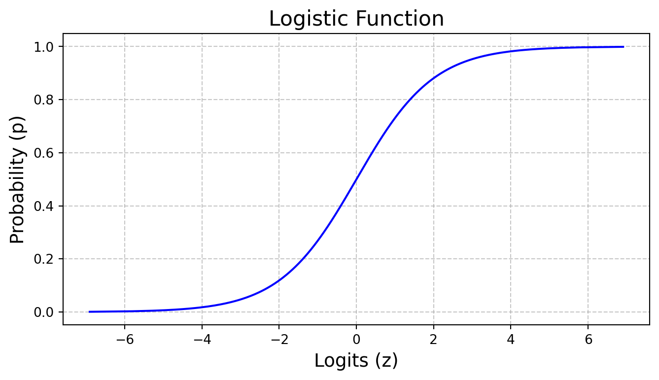
Awesome. We have ourselves a function that maps values from (0,1) to (-\infty,\infty). But what if we want the inverse? Map values from (-\infty,\infty) to (0,1). We simply take the inverse of the logit function. This yields the Logistic Function.
\begin{align*}
z &= \log_e{\frac{p}{1=p}} \\
e^z &= \frac{p}{1-p} \\
e^z (1-p) &= p \\
e^z - e^z p &= p \\
e^z &= p + e^z p \\
e^z &= p(1+e^z) \\
\frac{e^z}{(1+e^z)} &= p \\
p &= \frac{e^z}{(1+e^z)} \\
p &= \frac{1}{(1/e^z+1)} \\
p &= \frac{1}{(e^{-z}+1)}
\end{align*}
This below is a plot of the logistic function. This is also known as the sigmoid curve.
Code
import numpy as npimport pandas as pdimport seaborn as snsimport matplotlib.pyplot as plt# x valuesp = np.linspace(0.001, 0.999, 500)# calculate the logit function. np uses base e by default.logit_p = np.log(p / (1- p))logistic_p =1/(1+np.exp(-logit_p))data = pd.DataFrame({'logits (z)': logit_p, 'p': logistic_p})# plottingplt.figure(figsize=(8, 4))sns.lineplot(x='logits (z)', y='p', data=data, color='blue')plt.title('Logistic Function', fontsize=16)plt.xlabel('Logits (z)', fontsize=14)plt.ylabel('Probability (p)', fontsize=14)plt.grid(True, linestyle='--', alpha=0.7)plt.show()
Figure 2: Logistic function
So why go through all of this work of mapping values from one range to another? The main reason is so that we can enable linear modeling. Recall from linear regression, any value can be mapped to an output – linear regressions are unbounded. However, probabilities pose a challenge in that they are bounded between 0 and 1. The logit function solves this issue by transforming the probability space into log-odds. We can now predict log-odd values, which implicitly means we can predict probabilities.
Using a Logistic Regression Model
Consider a vector \theta in (d+1)-dimensional feature space. For any given point (x) in the feature space, we project it onto \theta to convert it into a real number z in the range (-\infty, \infty). z=\theta_0 + \theta_1 x_1 + \dots + \theta_d x_d.z=\theta \cdot x =\theta^T x. Now that we have z, we can map it to 0 to 1 using the logistic (sigmoid) function. p=y(x)=\sigma(z) = \frac{1}{1+e^{-z}}.
For example, let’s condier a first-order model.
z=\theta_0 + \theta_1 x_1.
p = \sigma(z) = \frac{1}{1+e^{-(\theta_0 + \theta_1 x_1)}}. Oh look! A linear regression tucked away in our logistic function.
So with p being a value between 0 and 1, we can model class probability. More formally,
p(C=1 | x) = \sigma(\theta^Tx) = \frac{1}{1+e^{-\theta^Tx}} with \sigma(z)=\frac{1}{1+e^{-z}}.
In a binary classification case, p(C=0|x) can be modeled as the complement of p(C=1|x). So, p(C=0|x) = 1-p(C=1|x) = 1-\frac{1}{1+e^{-\theta^Tx}} = \frac{e^{-\theta^Tx}}{1+e^{-\theta^Tx}}.
Finding the Best Parameters with MLE 🧐
We have the model but how do we find the optimal parameters, \theta\;? We use maximum likelihood estimation (MLE).
If the actual label y^{(i)} is true, the equation becomes P(y^{(i) = +1 | x^{(i)};\theta}) = \frac{1}{1+e^{-\theta^T x}}.
Otherwise, the equation becomes P(y^{(i) = -1 | x^{(i)};\theta}) = 1-\frac{1}{1+e^{-\theta^T x}}. Note that the in the binary case, we can set the decision boundary to 0.5. This is when \theta^Tx=0. Thus for the binary case, p(y^{(i)}|x^{(i);\theta}) = (p_i)^{y^{(i)}}(1-p_i)^{1-y^{(i)}}.
Plugging in the marginal probability property, we get
\begin{align*}
\text{max}_\theta \; \ell\ell(w) &= \text{max}_\theta \sum_i \log{P(y^{(i)} | x^{(i)}; \theta)} \\
&= \text{max}_\theta \sum_i \log{((p_i)^{y^{(i)}}(1-p_i)^{1-y^{(i)}})} \\
&= \text{max}_\theta \sum_i y^{(i)}\log{p_i} + (1-y^{(i)})\log{(1-p_i)}
\end{align*}
and that’s the final expression for log-likelihood! We can use Gradient Descent (GD) to find the parameters. The derived formula says max, but GD makes the loss as small as possible. To address GD finding the minimum optimum, we negate the loss function.
The gradients themselves are derived by applying the chain rule to the log-loss function. The log-loss function (L) itself contains the sigmoid function (p=\sigma(z)); inside the sigmoid function is the linear function (z). Going from out to in, we take the partial derivative using the chain rule. \frac{\partial L}{\partial w_j} = \frac{\partial L}{\partial p}\cdot \frac{\partial p}{\partial z}\cdot \frac{\partial z}{\partial w_j}.
I’ll leave the derivation as an exercise to the audience. However, I highly encourage it! This is one of the most elegant derivations in machine learning - setting the stage for more advanced techniques. Any computer science student taking a machine learning course should at least do the full derivative once throughout their academic journey.
Hence, binary cross entropy loss (often averaged over all samples) becomes Loss = -\frac{1}{N}\sum_{i=1}^N[y^{(i)}\log{(p_i)} + (1-y^{(i)})\log{1-p_i}].
Baseball Application
Earlier this season, Statcast published their swing path data on baseballsavant. Three new metrics were introduced: attack angle, attack direction, and swing path tilt. What is special about these new statistics is their level of granularity in measuring a bat swing. It is similar to how indoor golf studios are equipped with all sorts of sensors to track your golf swing (minus the ridiculous upcharge for a 30-min golf lesson).
In messing around with the eye-catching visuals on Baseball Savant, I noticed a dichotomous pattern among batters and their ideal attack angle rate and hard-hit outcome. Take a look at the distribution of batted balls grouped by if they were hard hit. We see a distinct distribution depending on the ideal attack angle rate.
Code
import pandas as pdimport seaborn as snssns.set_theme()df = pd.read_csv("bat-tracking-swing-path-year.csv")s = sns.kdeplot(data=df, x="ideal_attack_angle_rate", hue="is_hit_into_play_hardhit", fill=True)s.set_xlabel("Ideal Attack Angle Rate")s.set_title("Distribution of Hard Hit Outcomes Given Ideal Attack Angle Rate")plt.legend(title='Hard Hit', loc='upper right', labels=['Yes', 'No'])
Figure 3: KDE plots of batted ball with ideal attack angle rate and hard hit outcome.
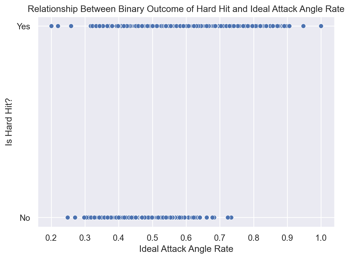
Observe the plot below. The x-axis measures the ideal attack angle rate: a metric indicating how consistently a batter achieves their optimal launch angle. The y-axis is binary: 1 if the ball was hard-hit (typically defined as 95+ mph exit velocity), 0 otherwise. Let’s apply a logistic regression to measure how strongly ideal attack angle rate predicts hard-hit probability, estimate the rate at which the probability transitions, and make probabilistic predictions on new data.
Code
s = sns.scatterplot(data=df, x="ideal_attack_angle_rate", y="is_hit_into_play_hardhit")s.set_ylabel("Is Hard Hit?")s.set_xlabel("Ideal Attack Angle Rate")s.set_yticks([0, 1])s.set_yticklabels(["No", "Yes"])s.set_title("Relationship Between Binary Outcome of Hard Hit and Ideal Attack Angle Rate");
Figure 4: Scatter plots of batted ball with ideal attack angle rate and hard hit outcome.
We build a logistic regression model from scratch.
Code
import numpy as npfrom sklearn.preprocessing import StandardScalerimport matplotlib.pyplot as pltclass LogisticRegressionScratch:"""Make class for logistic regression model built from scratch using NumPy."""def__init__(self, lr=0.01, n_iters=1000):self.lr = lrself.n_iters = n_itersself.weights =Noneself.bias =Nonedef _sigmoid(self, z):"""Call sigmoid activation function."""return1/ (1+ np.exp(-z))def fit(self, X, y):""" Train the model using gradient descent.""" n_samples, n_features = X.shape# 1. Initialize parametersself.weights = np.zeros(n_features)self.bias =0# 2. Gradient Descentfor _ inrange(self.n_iters):# Calculate the linear model output linear_model = np.dot(X, self.weights) +self.bias# Apply the sigmoid function to get probabilities y_predicted =self._sigmoid(linear_model)# Calculate the gradients dw = (1/ n_samples) * np.dot(X.T, (y_predicted - y)) db = (1/ n_samples) * np.sum(y_predicted - y)# Update the parametersself.weights -=self.lr * dwself.bias -=self.lr * dbdef predict(self, X):"""Make predictions on new data.""" linear_model = np.dot(X, self.weights) +self.bias y_predicted =self._sigmoid(linear_model) y_predicted_cls = [1if i >0.5else0for i in y_predicted]return np.array(y_predicted_cls)X = df[["ideal_attack_angle_rate"]].valuesy = df["is_hit_into_play_hardhit"].valuesscaler = StandardScaler()X_scaled = scaler.fit_transform(X)# init modelmodel = LogisticRegressionScratch(lr=0.01, n_iters=10000)model.fit(X_scaled, y)print(f"Learned Weights: {model.weights[0]:.4f}")print(f"Learned Bias: {model.bias:.4f}")
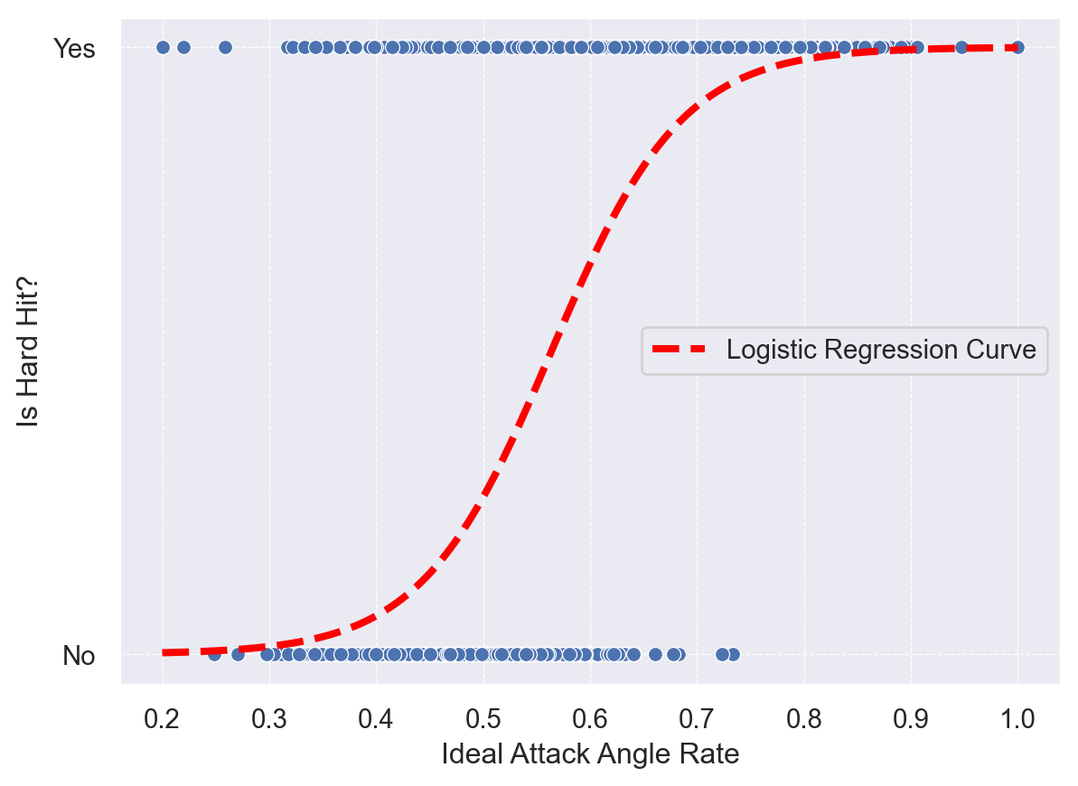
The red S-shaped curve on the plot is the model’s prediction. For any given “Ideal Attack Angle Rate” on the x-axis, the curve’s height on the y-axis represents the predicted probability of that swing resulting in a hard-hit ball.
Where the curve is low, the model predicts a low probability of a hard hit.
Where the curve is high, the model predicts a high probability of a hard hit.
The most important point on this curve is the decision boundary, where the probability is exactly 0.5. This is the threshold where the model’s prediction flips from “No” (less than 50% chance) to “Yes” (greater than 50% chance). We can calculate this exact point: it occurs where the linear function z=w⋅x+b is zero. For our model trained on scaled data, this gives us the crossover point for a player’s ideal attack angle rate.
To get a more precise understanding, we need to look at the math. A logistic regression model is a linear model for the log-odds of an event. \log{(\frac{p}{1-p})=w\cdot x + b} This equation tells us how the learned weight and bias directly impact those odds. To make the weight intuitive, we convert it from log-odds to an odds ratio by calculating e^w.
Let’s use the weight our model learned on the scaled data (e.g., a weight of 2.1455). \text{Odds ratio} = e^{2.1455} \approx 8.57. For every one standard deviation increase in a player’s ideal_attack_angle_rate, the odds of them getting a hard hit multiply by approximately 8.57.
The bias is 0.1103. This means the odds of a player with an average ideal attack angle rate hitting the ball hard is e^{0.1103} \approx 1.116. This means that for a player with an average ideal attack angle rate, the odds of them hitting the ball hard is about 1.116 to 1, or a 53% chance.
Scikit-Learn Example
Last but not least, let’s run sklearn to validate our findings. When given a raw dataset you are going to train a model on, you should always split the data into training and testing sets. This ensures that your model is not overfitting to the training data and can generalize well to unseen data.
import numpy as npfrom sklearn.model_selection import train_test_splitfrom sklearn import datasetsX = df[['ideal_attack_angle_rate']]y = df['is_hit_into_play_hardhit']print(f"Raw data shapes: features {X.shape}, labels {y.shape}")X_train, X_test, y_train, y_test = train_test_split(X, y, test_size=0.2, random_state=47)test_indices = X_test.index # to recall laterprint(f"Train data shapes: features {X_train.shape}, labels {y_train.shape}")print(f"Test data shapes: features {X_test.shape}, labels {y_test.shape}")
Raw data shapes: features (1134, 1), labels (1134,)
Train data shapes: features (907, 1), labels (907,)
Test data shapes: features (227, 1), labels (227,)
Next, we should clean the data. We will scale the ideal attack angle rate features; this makes our data more normalized.
Now we can fit the model. However, what happens if we overfit on the training data? We can use cross-validation to ensure that our model is robust and generalizes well.
cv = KFold(n_splits=5, shuffle=True, random_state=47)cv_scores = cross_val_score(pipeline, X_train, y_train, cv=cv, scoring='accuracy')print(f"K-Fold Cross-Validation Scores: {np.round(cv_scores, 3)}")print(f"Average CV Score: {cv_scores.mean():.3f} (+/- {cv_scores.std():.3f})")print("-"*40)# Now, train the final model on the ENTIRE training set.pipeline.fit(X_train, y_train)y_pred = pipeline.predict(X_test)final_accuracy = accuracy_score(y_test, y_pred)print(f"Final Test Set Accuracy: {final_accuracy:.3f}")
K-Fold Cross-Validation Scores: [0.797 0.841 0.818 0.79  0.807]
Average CV Score: 0.810 (+/- 0.018)
----------------------------------------
Final Test Set Accuracy: 0.802
80% accuracy is an ok result for a model trained on a single feature. Now let’s look at the coefficients to see how significant the ideal attack angle rate is.
model = pipeline.named_steps['model']coef = model.coef_[0]intercept = model.intercept_[0]print(f"Coefficient for Ideal Attack Angle Rate: {coef[0]:.4f}")print(f"Intercept: {intercept:.4f}")odds_ratios = np.exp(coef)for name, odds inzip(["Ideal Attack Angle Rate"], odds_ratios):print(f"Odds Ratio for {name}: {odds:.3f}")print("-"*40)
Coefficient for Ideal Attack Angle Rate: 2.1094
Intercept: 0.0900
Odds Ratio for Ideal Attack Angle Rate: 8.244
----------------------------------------
An odds ratio of 8.244, which we get by computing (e^{2.1094}), means that for every one standard deviation increase in a player’s ideal attack angle rate, the odds of them hitting the ball hard multiply by approximately 8.244. This is a significant relationship, indicating that this feature is a strong predictor of hard-hit outcomes. The intercept of 0.0900 suggests that for a player with an average ideal attack angle rate, the odds of hitting the ball hard are about 1.094 to 1, or a 52.2% chance.
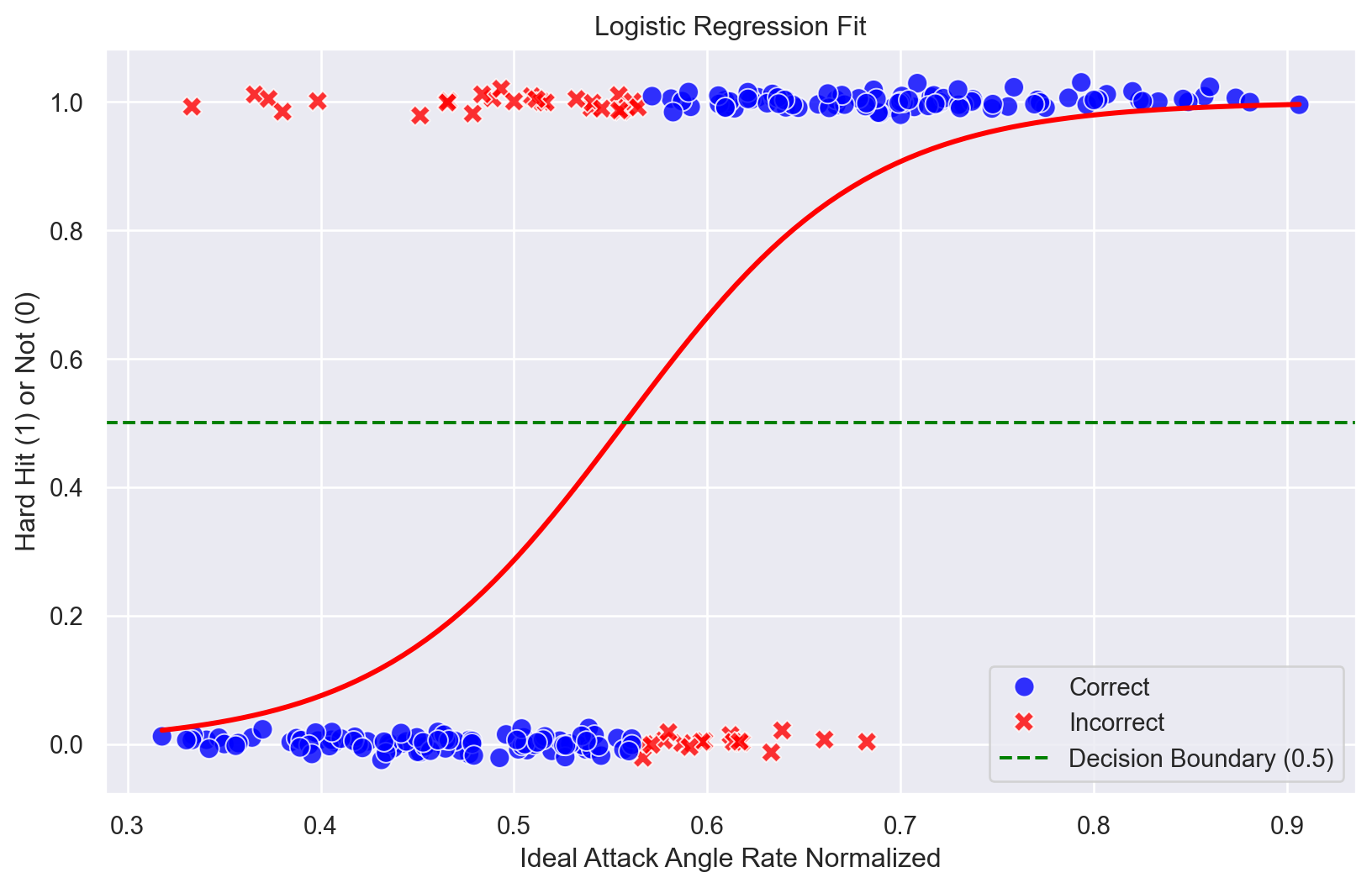
Finally, let’s visualize the model’s predictions on the test set.
Code
import seaborn as snsimport matplotlib.pyplot as pltimport pandas as pdimport numpy as np# testnp.random.seed(47)y_pred_proba = pipeline.predict_proba(X_test)[:, 1]y_pred_proba = (y_pred_proba >0.5).astype(int)# --- Create DataFrame and Plot with Seaborn ---# Combine the actual outcomes and the feature into a DataFramedf_test = pd.DataFrame({'Ideal Attack Angle Rate': X_test.values.flatten(),'Hard Hit Actual': y_test,})df_test['Result'] = np.where(df_test['Hard Hit Actual'] == y_pred_proba, 'Correct', 'Incorrect')plt.figure(figsize=(10, 6))# Use regplot to show the data points and the fitted logistic curvesns.regplot( x='Ideal Attack Angle Rate', y='Hard Hit Actual', data=df_test, logistic=True, ci=None, # Turn off confidence interval for this plot y_jitter=.03, scatter_kws={'alpha': 0.5, 'color': 'blue'}, line_kws={'color': 'red', 'label': 'Fitted Logistic Curve'}, scatter=False,)def jitter(values,j):return values + np.random.normal(j,0.01,values.shape)0df_test['Hard Hit Actual'] = jitter(df_test['Hard Hit Actual'], 0.001)sns.scatterplot( x='Ideal Attack Angle Rate', y='Hard Hit Actual', hue='Result', style='Result', # Use different markers for correctness palette={'Correct': 'blue', 'Incorrect': 'red'}, data=df_test, s=80, alpha=0.8)plt.axhline(0.5, color='green', linestyle='--', label='Decision Boundary (0.5)')plt.title('Logistic Regression Fit')plt.ylabel('Hard Hit (1) or Not (0)')plt.xlabel('Ideal Attack Angle Rate Normalized')plt.legend()plt.show()
Figure 5: Logistic Regression Predictions on Test Set
Pretty cool stuff. The red points represent the model’s predictions, while the blue points are the actual labels. The green dashed line indicates the decision boundary at 0.5, where the model predicts a hard hit.
Of course, we can’t win them all. Some players will have swings that don’t translate to hard hits, even if they have a high ideal attack angle rate. Those players are shown in the table below. These are the model misclassifications.
Everyone in the game, from the front-office Ivy Leaguers to the Silicon Valley startups trying to sell them something, loves to type .fit() and watch the magic happen. They get an answer, they nod, and they move on. But they have no earthly idea what’s going on inside the box. They’re flying a 747 on autopilot without ever having seen the cockpit.
So we decided to pry the thing open. We went back to the beginning, to the raw, messy mathematics of a logistic regression. Inside, we found this relentless engine called Maximum Likelihood Estimation, a fancy term for a machine built to find the single most plausible story for what the hell is going on in the data. We watched it work, watched the gradients crawl their way down the mountain, each step a tiny, agonizing calculation on the path to the best possible answer. It wasn’t elegant, but it was honest.
Once you’ve built the engine, you want to see what it can do. You want to point it at something. We pointed it at baseball. We fed it a mountain of swing data, and the machine started to hum.
And then it spit out a signal, a signal so loud it was impossible to ignore. Forget what the scouts told you about a “pretty swing.” One number mattered more than the others: ideal_attack_angle_rate. It was right there in the data, a clear, blinking light showing that the players who got their bat on the perfect plane to meet the ball weren’t just making better contact—they were hitting the ball hard.
But here’s the beautiful part. The model didn’t just tell us the two things were connected. It told us the price. It handed us a number that said for every standard deviation a player improved in this one metric—a totally learnable skill—the odds that he’d lace a ball into the gap went up by a multiplier that could change the course of a franchise.
This is the point where you realize logistic regression isn’t just some sorting hat for data. It’s a pair of X-ray specs. It lets you look past the noise and see the hidden architecture of a problem. It gives you an edge that is not only predictive, but that you can actually understand and explain.
Don’t believe me? Go pull up a video of Corbin Carroll hitting a triple. He’s third in the league in ideal attack angle. The machine saw him coming.
Source Code
---title: "Logistic Regression"author: "Oliver Chang"email: oliverc1622@gmail.comdate: "2025-07-11"categories: [numpy, classification, MLB]image: "attack-angle.png"format: html: html-math-method: katex code-tools: true---<iframe src="https://streamable.com/m/dat-viz-juan-soto-s-two-run-home-run?partnerId=web_video-playback-page_video-share" width="720" height="415"></iframe># IntroductionLast [article](https://runningonnumbers.com/posts/ops-linear-regression/), we introduced linear regression and applied it to predict MLB teams' runs scored given OPS. Linear regression is great at predicting numerical values. For example, it can predict runs scored given OPS. However, what happens if we want to move away from predicting continuous values and do binary classification? How can we predict whether a batter's swing mechanics will result in a ["hard-hit"](https://www.mlb.com/glossary/statcast/hard-hit-rate) batted ball? We are going to have to turn to logistic regression!Contrary to its name, logistic regression is a classification technique (you will see where the regression part comes from). Logistic regression involves a probabilistic view of classification. This binary classification method maps a data point to a probabilistic value in the range 0 to 1. Let's dig into some mathematical formalities.# Logistic Regression## Preliminaries"Never tell me the odds" - Han Solo.The average movie watcher could hear this quote with a slight alteration, where the word "odds" is replaced by "probability," and they would not bat an eye. However, a statistician would have an issue with substituting the word "odds" with "probability." While in layman terms they both share similar meaning, in mathematics they are defined distinctly.Odds are a transformation of probabilities - they are another way to think about probabilities. More formally, $$\text{odds} = \frac{p}{1-p}$$where $p$ denotes some probability value between 0 and 1, and $1-p$ denotes the complement. Think of it as the probability of something happening divided by the probability of it not happening. If given some event, $E$, where the odds are $x$ to $y$, then that means $Odds(E)=\frac{x}{y}$. Subsequently, $P(E)=\frac{x}{x+y}$. The range of possible values for odds becomes 0 to $\infty$. When using probability values between 0 and 1, the range of odds becomes (0,1). Observe that this is an open interval. If $p=1$, then the denominator becomes $1-1 = 0$. We cannot divide by zero, so the upper bound is undefined at 1. When $p=0$, we get $\frac{0}{1}=0$. If we are going to do any regressions of this sort, we will need to expand our real number bounds.To get an unbounded range, we introduce the logit function. The logit function takes in a value between 0 and 1 and maps it to a value between $-\infty$ and $\infty$. $$z = \log_e{\frac{p}{1-p}}.$$Below is a plot for what the logit function looks like.```{python}#| code-fold: true#| warning: false#| label: fig-logit#| fig-cap: Logit functionimport numpy as npimport pandas as pdimport seaborn as snsimport matplotlib.pyplot as plt# x valuesp = np.linspace(0.001, 0.999, 500)# calculate the logit function. np uses base e by default.logit_p = np.log(p / (1- p))data = pd.DataFrame({'Probability (p)': p, 'Logit(p)': logit_p})# plottingplt.figure(figsize=(8, 4))sns.lineplot(x='Probability (p)', y='Logit(p)', data=data, color='blue')plt.title('Logit Function', fontsize=16)plt.xlabel('Probability (p)', fontsize=14)plt.ylabel('Logit(p) = ln(p / (1 - p))', fontsize=14)plt.grid(True, linestyle='--', alpha=0.7)plt.show()```Awesome. We have ourselves a function that maps values from (0,1) to $(-\infty,\infty)$. But what if we want the inverse? Map values from $(-\infty,\infty)$ to $(0,1).$ We simply take the inverse of the logit function. This yields the **Logistic Function.**$$\begin{align*} z &= \log_e{\frac{p}{1=p}} \\ e^z &= \frac{p}{1-p} \\ e^z (1-p) &= p \\ e^z - e^z p &= p \\ e^z &= p + e^z p \\ e^z &= p(1+e^z) \\ \frac{e^z}{(1+e^z)} &= p \\ p &= \frac{e^z}{(1+e^z)} \\ p &= \frac{1}{(1/e^z+1)} \\ p &= \frac{1}{(e^{-z}+1)}\end{align*}$$This below is a plot of the logistic function. This is also known as the sigmoid curve.```{python}#| code-fold: true#| warning: false#| label: fig-logistic#| fig-cap: Logistic functionimport numpy as npimport pandas as pdimport seaborn as snsimport matplotlib.pyplot as plt# x valuesp = np.linspace(0.001, 0.999, 500)# calculate the logit function. np uses base e by default.logit_p = np.log(p / (1- p))logistic_p =1/(1+np.exp(-logit_p))data = pd.DataFrame({'logits (z)': logit_p, 'p': logistic_p})# plottingplt.figure(figsize=(8, 4))sns.lineplot(x='logits (z)', y='p', data=data, color='blue')plt.title('Logistic Function', fontsize=16)plt.xlabel('Logits (z)', fontsize=14)plt.ylabel('Probability (p)', fontsize=14)plt.grid(True, linestyle='--', alpha=0.7)plt.show()```So why go through all of this work of mapping values from one range to another? The main reason is so that we can enable linear modeling. Recall from [linear regression](https://runningonnumbers.com/posts/ops-linear-regression/), any value can be mapped to an output – linear regressions are unbounded. However, probabilities pose a challenge in that they are bounded between 0 and 1. The logit function solves this issue by transforming the probability space into log-odds. We can now predict log-odd values, which implicitly means we can predict probabilities.## Using a Logistic Regression ModelConsider a vector $\theta$ in (d+1)-dimensional feature space. For any given point ($x$) in the feature space, we project it onto $\theta$ to convert it into a real number $z$ in the range ($-\infty, \infty$). $z=\theta_0 + \theta_1 x_1 + \dots + \theta_d x_d.$ $z=\theta \cdot x =\theta^T x.$ Now that we have $z$, we can map it to 0 to 1 using the logistic (sigmoid) function. $p=y(x)=\sigma(z) = \frac{1}{1+e^{-z}}.$For example, let's condier a first-order model.$z=\theta_0 + \theta_1 x_1.$$p = \sigma(z) = \frac{1}{1+e^{-(\theta_0 + \theta_1 x_1)}}.$ Oh look! A linear regression tucked away in our logistic function.So with $p$ being a value between 0 and 1, we can model class probability. More formally, $$p(C=1 | x) = \sigma(\theta^Tx) = \frac{1}{1+e^{-\theta^Tx}}$$with $\sigma(z)=\frac{1}{1+e^{-z}}.$In a binary classification case, $p(C=0|x)$ can be modeled as the complement of $p(C=1|x)$. So, $p(C=0|x) = 1-p(C=1|x) = 1-\frac{1}{1+e^{-\theta^Tx}} = \frac{e^{-\theta^Tx}}{1+e^{-\theta^Tx}}.$### Finding the Best Parameters with MLE 🧐We have the model but how do we find the optimal parameters, $\theta\;$? We use maximum likelihood estimation (MLE). MLE:$$\text{max}_\theta \; \ell\ell(w)=\text{max}_\theta \sum_i \log{P(y^{(i)} | x^{(i)}; \theta)}.$$If the actual label $y^{(i)}$ is true, the equation becomes $P(y^{(i) = +1 | x^{(i)};\theta}) = \frac{1}{1+e^{-\theta^T x}}.$Otherwise, the equation becomes $P(y^{(i) = -1 | x^{(i)};\theta}) = 1-\frac{1}{1+e^{-\theta^T x}}$. Note that the in the binary case, we can set the decision boundary to 0.5. This is when $\theta^Tx=0.$ Thus for the binary case, $p(y^{(i)}|x^{(i);\theta}) = (p_i)^{y^{(i)}}(1-p_i)^{1-y^{(i)}}.$Plugging in the marginal probability property, we get$$\begin{align*}\text{max}_\theta \; \ell\ell(w) &= \text{max}_\theta \sum_i \log{P(y^{(i)} | x^{(i)}; \theta)} \\ &= \text{max}_\theta \sum_i \log{((p_i)^{y^{(i)}}(1-p_i)^{1-y^{(i)}})} \\ &= \text{max}_\theta \sum_i y^{(i)}\log{p_i} + (1-y^{(i)})\log{(1-p_i)}\end{align*}$$and that's the final expression for log-likelihood! We can use Gradient Descent (GD) to find the parameters. The derived formula says `max`, but GD makes the loss as small as possible. To address GD finding the minimum optimum, we negate the loss function.The gradients themselves are derived by applying the chain rule to the log-loss function. The log-loss function ($L$) itself contains the sigmoid function ($p=\sigma(z)$); inside the sigmoid function is the linear function ($z$). Going from out to in, we take the partial derivative using the chain rule.$$\frac{\partial L}{\partial w_j} = \frac{\partial L}{\partial p}\cdot \frac{\partial p}{\partial z}\cdot \frac{\partial z}{\partial w_j}.$$I'll leave the derivation as an exercise to the audience. However, I highly encourage it! This is one of the most elegant derivations in machine learning - setting the stage for more advanced techniques. Any computer science student taking a machine learning course should at least do the full derivative once throughout their academic journey.Hence, binary cross entropy loss (often averaged over all samples) becomes$$Loss = -\frac{1}{N}\sum_{i=1}^N[y^{(i)}\log{(p_i)} + (1-y^{(i)})\log{1-p_i}].$$# Baseball ApplicationEarlier this season, Statcast published their swing path data on [baseballsavant](https://baseballsavant.mlb.com/leaderboard/bat-tracking/swing-path-attack-angle). Three new metrics were introduced: attack angle, attack direction, and swing path tilt. What is special about these new statistics is their level of granularity in measuring a bat swing. It is similar to how indoor golf studios are equipped with all sorts of sensors to track your golf swing (minus the ridiculous upcharge for a 30-min golf lesson).In messing around with the eye-catching visuals on Baseball Savant, I noticed a dichotomous pattern among batters and their *ideal attack angle rate* and *hard-hit* outcome. Take a look at the distribution of batted balls grouped by if they were hard hit. We see a distinct distribution depending on the ideal attack angle rate. ```{python}#| code-fold: true#| warning: false#| label: fig-kde-ideal-attack-angle-rate#| fig-cap: KDE plots of batted ball with ideal attack angle rate and hard hit outcome.import pandas as pdimport seaborn as snssns.set_theme()df = pd.read_csv("bat-tracking-swing-path-year.csv")s = sns.kdeplot(data=df, x="ideal_attack_angle_rate", hue="is_hit_into_play_hardhit", fill=True)s.set_xlabel("Ideal Attack Angle Rate")s.set_title("Distribution of Hard Hit Outcomes Given Ideal Attack Angle Rate")plt.legend(title='Hard Hit', loc='upper right', labels=['Yes', 'No'])```Observe the plot below. The x-axis measures the ideal attack angle rate: a metric indicating how consistently a batter achieves their optimal launch angle. The y-axis is binary: 1 if the ball was hard-hit (typically defined as 95+ mph exit velocity), 0 otherwise. Let's apply a logistic regression to measure how strongly ideal attack angle rate predicts hard-hit probability, estimate the rate at which the probability transitions, and make probabilistic predictions on new data.```{python}#| code-fold: true#| warning: false#| label: fig-empirical-log#| fig-cap: Scatter plots of batted ball with ideal attack angle rate and hard hit outcome.s = sns.scatterplot(data=df, x="ideal_attack_angle_rate", y="is_hit_into_play_hardhit")s.set_ylabel("Is Hard Hit?")s.set_xlabel("Ideal Attack Angle Rate")s.set_yticks([0, 1])s.set_yticklabels(["No", "Yes"])s.set_title("Relationship Between Binary Outcome of Hard Hit and Ideal Attack Angle Rate");```We build a logistic regression model from scratch.```{python}#| code-fold: true#| warning: falseimport numpy as npfrom sklearn.preprocessing import StandardScalerimport matplotlib.pyplot as pltclass LogisticRegressionScratch:"""Make class for logistic regression model built from scratch using NumPy."""def__init__(self, lr=0.01, n_iters=1000):self.lr = lrself.n_iters = n_itersself.weights =Noneself.bias =Nonedef _sigmoid(self, z):"""Call sigmoid activation function."""return1/ (1+ np.exp(-z))def fit(self, X, y):""" Train the model using gradient descent.""" n_samples, n_features = X.shape# 1. Initialize parametersself.weights = np.zeros(n_features)self.bias =0# 2. Gradient Descentfor _ inrange(self.n_iters):# Calculate the linear model output linear_model = np.dot(X, self.weights) +self.bias# Apply the sigmoid function to get probabilities y_predicted =self._sigmoid(linear_model)# Calculate the gradients dw = (1/ n_samples) * np.dot(X.T, (y_predicted - y)) db = (1/ n_samples) * np.sum(y_predicted - y)# Update the parametersself.weights -=self.lr * dwself.bias -=self.lr * dbdef predict(self, X):"""Make predictions on new data.""" linear_model = np.dot(X, self.weights) +self.bias y_predicted =self._sigmoid(linear_model) y_predicted_cls = [1if i >0.5else0for i in y_predicted]return np.array(y_predicted_cls)X = df[["ideal_attack_angle_rate"]].valuesy = df["is_hit_into_play_hardhit"].valuesscaler = StandardScaler()X_scaled = scaler.fit_transform(X)# init modelmodel = LogisticRegressionScratch(lr=0.01, n_iters=10000)model.fit(X_scaled, y)print(f"Learned Weights: {model.weights[0]:.4f}")print(f"Learned Bias: {model.bias:.4f}")```Using the weights, let's plot the sigmoid curve.```{python}#| code-fold: true#| warning: falses = sns.scatterplot(data=df, x="ideal_attack_angle_rate", y="is_hit_into_play_hardhit")s.set_ylabel("Is Hard Hit?")s.set_xlabel("Ideal Attack Angle Rate")s.set_yticks([0, 1])s.set_yticklabels(["No", "Yes"])x_curve = np.linspace(df["ideal_attack_angle_rate"].min(), df["ideal_attack_angle_rate"].max(), 200).reshape(-1, 1)x_curve_scaled = scaler.transform(x_curve)z_curve = np.dot(x_curve_scaled, model.weights) + model.biasy_curve = model._sigmoid(z_curve)plt.plot(x_curve, y_curve, color='red', linestyle="--", linewidth=3, label='Logistic Regression Curve')plt.legend()plt.grid(True, which='both', linestyle='--', linewidth=0.5)plt.show()```The red S-shaped curve on the plot is the model's prediction. For any given "Ideal Attack Angle Rate" on the x-axis, the curve's height on the y-axis represents the predicted probability of that swing resulting in a hard-hit ball.- Where the curve is low, the model predicts a low probability of a hard hit.- Where the curve is high, the model predicts a high probability of a hard hit.The most important point on this curve is the decision boundary, where the probability is exactly 0.5. This is the threshold where the model's prediction flips from "No" (less than 50% chance) to "Yes" (greater than 50% chance). We can calculate this exact point: it occurs where the linear function z=w⋅x+b is zero. For our model trained on scaled data, this gives us the crossover point for a player's ideal attack angle rate.To get a more precise understanding, we need to look at the math. A logistic regression model is a linear model for the log-odds of an event.$\log{(\frac{p}{1-p})=w\cdot x + b}$This equation tells us how the learned weight and bias directly impact those odds. To make the weight intuitive, we convert it from log-odds to an odds ratio by calculating $e^w$. Let's use the weight our model learned on the scaled data (e.g., a weight of 2.1455). $\text{Odds ratio} = e^{2.1455} \approx 8.57$. For every one standard deviation increase in a player's ideal_attack_angle_rate, the odds of them getting a hard hit multiply by approximately 8.57.The bias is 0.1103. This means the odds of a player with an average ideal attack angle rate hitting the ball hard is $e^{0.1103} \approx 1.116$. This means that for a player with an average ideal attack angle rate, the odds of them hitting the ball hard is about 1.116 to 1, or a 53% chance.## Scikit-Learn ExampleLast but not least, let's run `sklearn` to validate our findings. When given a raw dataset you are going to train a model on, you should always split the data into training and testing sets. This ensures that your model is not overfitting to the training data and can generalize well to unseen data.```{python}#| code-fold: false#| warning: falseimport numpy as npfrom sklearn.model_selection import train_test_splitfrom sklearn import datasetsX = df[['ideal_attack_angle_rate']]y = df['is_hit_into_play_hardhit']print(f"Raw data shapes: features {X.shape}, labels {y.shape}")X_train, X_test, y_train, y_test = train_test_split(X, y, test_size=0.2, random_state=47)test_indices = X_test.index # to recall laterprint(f"Train data shapes: features {X_train.shape}, labels {y_train.shape}")print(f"Test data shapes: features {X_test.shape}, labels {y_test.shape}")```Next, we should clean the data. We will scale the ideal attack angle rate features; this makes our data more normalized. ```{python}#| code-fold: false#| warning: false from sklearn.preprocessing import StandardScalerfrom sklearn.pipeline import Pipelinefrom sklearn.linear_model import LogisticRegressionfrom sklearn.model_selection import KFold, cross_val_scorefrom sklearn.metrics import accuracy_scorepipeline = Pipeline([ ('scaler', StandardScaler()), ('model', LogisticRegression(random_state=47)),])```Now we can fit the model. However, what happens if we overfit on the training data? We can use cross-validation to ensure that our model is robust and generalizes well.```{python}cv = KFold(n_splits=5, shuffle=True, random_state=47)cv_scores = cross_val_score(pipeline, X_train, y_train, cv=cv, scoring='accuracy')print(f"K-Fold Cross-Validation Scores: {np.round(cv_scores, 3)}")print(f"Average CV Score: {cv_scores.mean():.3f} (+/- {cv_scores.std():.3f})")print("-"*40)# Now, train the final model on the ENTIRE training set.pipeline.fit(X_train, y_train)y_pred = pipeline.predict(X_test)final_accuracy = accuracy_score(y_test, y_pred)print(f"Final Test Set Accuracy: {final_accuracy:.3f}")```80% accuracy is an ok result for a model trained on a single feature. Now let's look at the coefficients to see how significant the ideal attack angle rate is.```{python}#| code-fold: false#| warning: falsemodel = pipeline.named_steps['model']coef = model.coef_[0]intercept = model.intercept_[0]print(f"Coefficient for Ideal Attack Angle Rate: {coef[0]:.4f}")print(f"Intercept: {intercept:.4f}")odds_ratios = np.exp(coef)for name, odds inzip(["Ideal Attack Angle Rate"], odds_ratios):print(f"Odds Ratio for {name}: {odds:.3f}")print("-"*40)```An odds ratio of 8.244, which we get by computing $(e^{2.1094})$, means that for every one standard deviation increase in a player's ideal attack angle rate, the odds of them hitting the ball hard multiply by approximately 8.244. This is a significant relationship, indicating that this feature is a strong predictor of hard-hit outcomes. The intercept of 0.0900 suggests that for a player with an average ideal attack angle rate, the odds of hitting the ball hard are about 1.094 to 1, or a 52.2% chance.Finally, let's visualize the model's predictions on the test set.```{python}#| code-fold: True#| warning: True#| label: fig-logistic-regression-plot#| fig-cap: Logistic Regression Predictions on Test Setimport seaborn as snsimport matplotlib.pyplot as pltimport pandas as pdimport numpy as np# testnp.random.seed(47)y_pred_proba = pipeline.predict_proba(X_test)[:, 1]y_pred_proba = (y_pred_proba >0.5).astype(int)# --- Create DataFrame and Plot with Seaborn ---# Combine the actual outcomes and the feature into a DataFramedf_test = pd.DataFrame({'Ideal Attack Angle Rate': X_test.values.flatten(),'Hard Hit Actual': y_test,})df_test['Result'] = np.where(df_test['Hard Hit Actual'] == y_pred_proba, 'Correct', 'Incorrect')plt.figure(figsize=(10, 6))# Use regplot to show the data points and the fitted logistic curvesns.regplot( x='Ideal Attack Angle Rate', y='Hard Hit Actual', data=df_test, logistic=True, ci=None, # Turn off confidence interval for this plot y_jitter=.03, scatter_kws={'alpha': 0.5, 'color': 'blue'}, line_kws={'color': 'red', 'label': 'Fitted Logistic Curve'}, scatter=False,)def jitter(values,j):return values + np.random.normal(j,0.01,values.shape)0df_test['Hard Hit Actual'] = jitter(df_test['Hard Hit Actual'], 0.001)sns.scatterplot( x='Ideal Attack Angle Rate', y='Hard Hit Actual', hue='Result', style='Result', # Use different markers for correctness palette={'Correct': 'blue', 'Incorrect': 'red'}, data=df_test, s=80, alpha=0.8)plt.axhline(0.5, color='green', linestyle='--', label='Decision Boundary (0.5)')plt.title('Logistic Regression Fit')plt.ylabel('Hard Hit (1) or Not (0)')plt.xlabel('Ideal Attack Angle Rate Normalized')plt.legend()plt.show()```Pretty cool stuff. The red points represent the model's predictions, while the blue points are the actual labels. The green dashed line indicates the decision boundary at 0.5, where the model predicts a hard hit.Of course, we can't win them all. Some players will have swings that don't translate to hard hits, even if they have a high ideal attack angle rate. Those players are shown in the table below. These are the model misclassifications.```{python}#| code-fold: True#| warning: Truemisclassified = df_test[df_test['Result'] =='Incorrect'].sort_values(by='Ideal Attack Angle Rate')df_joined = misclassified.join(df, how='inner', rsuffix='_misclassified')final_tbl = df_joined[['Ideal Attack Angle Rate', 'is_hit_into_play_hardhit', 'name']]final_tbl.head(5)```And here are the last 5 misclassifications.```{python}#| code-fold: True#| warning: falsefinal_tbl.tail(5)```# Conclusion: From Theory to InsightIt all starts with the black box.Everyone in the game, from the front-office Ivy Leaguers to the Silicon Valley startups trying to sell them something, loves to type .fit() and watch the magic happen. They get an answer, they nod, and they move on. But they have no earthly idea what’s going on inside the box. They’re flying a 747 on autopilot without ever having seen the cockpit.So we decided to pry the thing open. We went back to the beginning, to the raw, messy mathematics of a logistic regression. Inside, we found this relentless engine called Maximum Likelihood Estimation, a fancy term for a machine built to find the single most plausible story for what the hell is going on in the data. We watched it work, watched the gradients crawl their way down the mountain, each step a tiny, agonizing calculation on the path to the best possible answer. It wasn’t elegant, but it was honest.Once you’ve built the engine, you want to see what it can do. You want to point it at something. We pointed it at baseball. We fed it a mountain of swing data, and the machine started to hum.And then it spit out a signal, a signal so loud it was impossible to ignore. Forget what the scouts told you about a "pretty swing." One number mattered more than the others: ideal_attack_angle_rate. It was right there in the data, a clear, blinking light showing that the players who got their bat on the perfect plane to meet the ball weren't just making better contact—they were hitting the ball hard.But here’s the beautiful part. The model didn’t just tell us the two things were connected. It told us the price. It handed us a number that said for every standard deviation a player improved in this one metric—a totally learnable skill—the odds that he’d lace a ball into the gap went up by a multiplier that could change the course of a franchise.This is the point where you realize logistic regression isn't just some sorting hat for data. It's a pair of X-ray specs. It lets you look past the noise and see the hidden architecture of a problem. It gives you an edge that is not only predictive, but that you can actually understand and explain.Don’t believe me? Go pull up a video of Corbin Carroll hitting a triple. He’s third in the league in ideal attack angle. The machine saw him coming.<iframe src="https://streamable.com/m/trevor-williams-in-play-no-out-to-corbin-carroll-tdxvup?partnerId=web_video-playback-page_video-share" width="720" height="415"></iframe><script async data-uid="5d16db9e50" src="https://runningonnumbers.kit.com/5d16db9e50/index.js"></script>